
In our previous newsletter, we introduced Churn prediction using SAP SAP’s predictive scenarios tool. Now, we’re delving into feature engineering, a crucial step in machine learning. Following this, we’ll use Churn Prediction data with SAP SAC for practical application, demonstrating the power of our model in real-world scenarios.
What is feature engineering?
Feature engineering is the process of selecting, transforming, and creating new features from raw data to improve the performance of machine learning models. In the context of prediction, particularly classification tasks, feature engineering plays a crucial role in enhancing the model’s ability to accurately classify data points into different categories.
It is really important for a Machine Learning(ML) model for the main reasons:
Improves model performance: Improving the performance of classification models is possible through feature engineering. By carefully choosing relevant features and crafting new ones to highlight key patterns in the data, the model becomes more adept at distinguishing between different classes, resulting in higher accuracy, precision, and recall.
Reduce the noise of data: Raw data can have extra stuff that confuses the model and makes it overfit. Feature engineering helps by picking the important parts and changing them to show clear patterns while ignoring the unimportant stuff.
Dimension reduction: Feature selection methods help reduce the dimensionality.
Churn Prediction Model Development
In the previous example, we discussed the model’s results. Understanding both the data and the model’s outcomes is crucial for achieving better results in a data science project. The primary objective is to obtain the highest score, but achieving this doesn’t necessarily guarantee the best outcome. Some columns in the data may contain outliers or require adjustments, such as applying scaling methods like min-max or standard deviation.
As illustrated below, in the analysis of the first model’s influencer contributions, we observed that the “Age” column affects the model results by 30.17%.
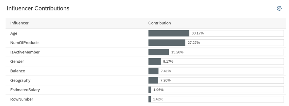
Since we’ve already removed outliers, let’s proceed with categorizing the age distribution to observe its effects and potentially enhance the model’s performance.
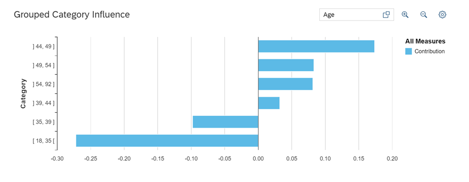
To categorize the age distribution into “Young,” “Adult,” and “Elderly” groups based on the specified age ranges (15-35, 35-45, and 45-65 respectively), follow these steps:
- Open the training dataset.
- Duplicate the age column to create a new column for the categorized age groups.
- Write the expression to assign each row to the appropriate group based on the specified age ranges.
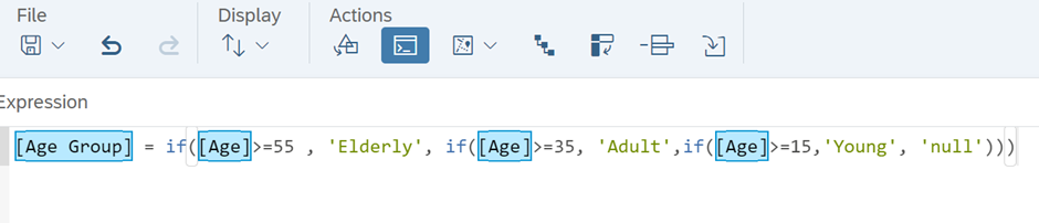
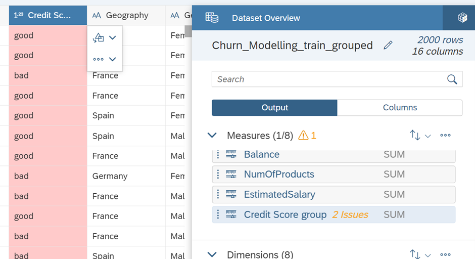
After validating and executing the expression, we might encounter an error because we’ve converted the integer column to a string. This warning needs to be addressed to utilize the grouped column in our model effectively.
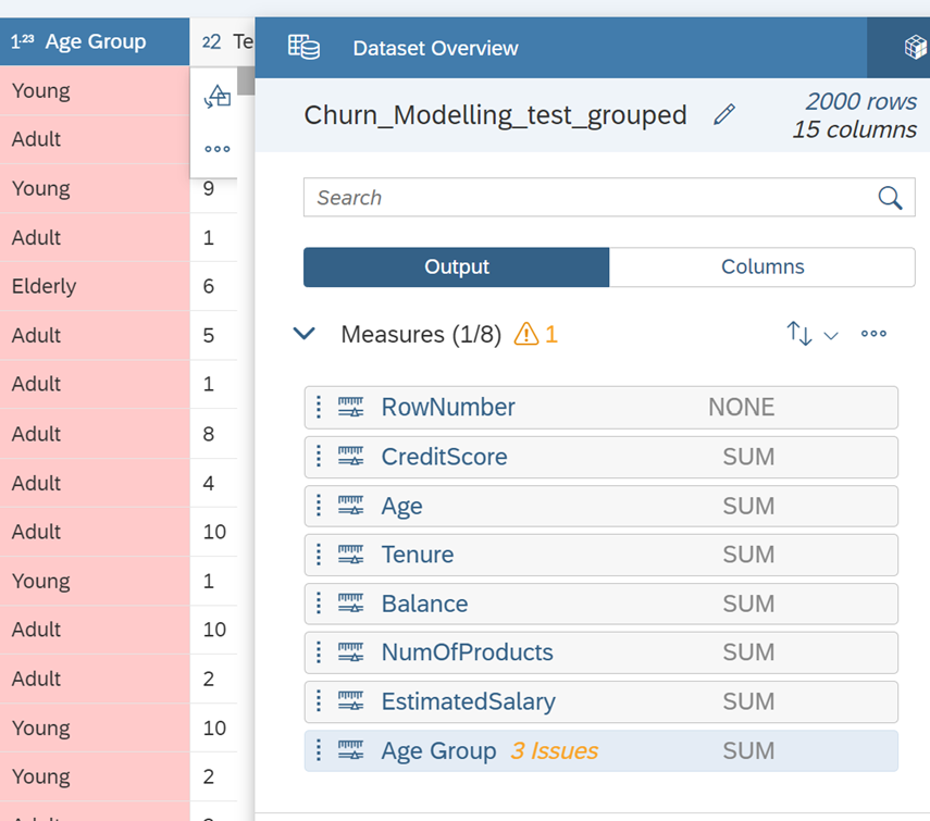
In this line, the data type has been changed from integer to string, causing the statistical type to transition from continuous to nominal. Furthermore, the ‘Credit Score’ column has been selected to introduce another grouping as a feature. After making these modifications, we’ll follow the same steps as depicted below to address the issues and assess the impact on the model by including and excluding them as influencers.
On the other hand, instead of using the ‘exit’ column as the target, a new column is created by applying an if clause as depicted to set the target. This column has a low effect on the solution. Therefore, we do not expect the accuracy of that model to be high, although we cannot make a final decision without trying it out.
Note: The same steps are applied to the test data as well.
Model Evaluation
The goal is to enhance the results from the previous week. To achieve this, we computed two additional classification models by changing the features. This exploration helps us gain a deeper understanding of the data and the working approach of machine learning models. Model 3 represents our previous model.
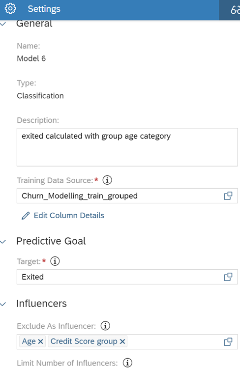
For Model 6, the ‘Age’ feature was excluded, and the ‘Credit score group’ column was removed from the model to prevent overtraining.
In addition to Model 6, in order to explore another potential scenario, credit score information is also excluded from Model 8. This means that Model 8 does not contain any credit score information. The main reason for this selection is that the credit score feature had the lowest impact as an influencer in the first model.
Model 7 represents the classification model’s performance based on the ‘Category score group’ column that we previously created. It turns out to be the worst-performing model when considering accuracy scores such as Gini index and classification rate, which is not unexpected.
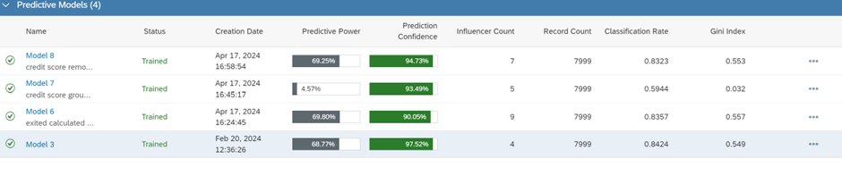
Despite slight differences in the evaluation parameters among the classification models (Model 3, Model 6, Model 8), Model 6 is selected as the optimal model. This decision is based on its higher Gini score, which is a more statistical approach, and its overall greater predictive power compared to the others.
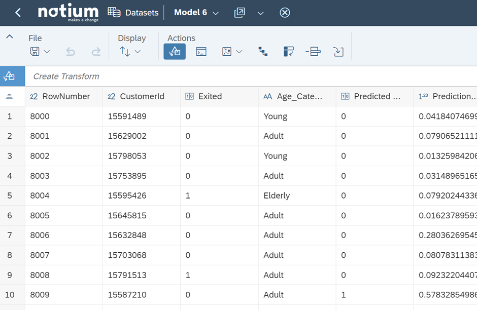
After the selection process, Model 6 was applied to the test data. Below are the first 10 columns of the test data, with the predicted probability column (6th) and the predicted category being the results generated by Model 6.
Conclusion
In this newsletter, we delved into the process of computing feature engineering, exploring various approaches of an ML Model, and developing predictive scenarios in SAP SAC using case scenarios. SAP SAC offers a user-friendly interface even for complex prediction scenarios. Apart from classification, it also provides tools for time-series analysis and regression, which we’ll cover in our upcoming newsletter.