
In our previous newsletters, we explored the predictive scenarios in SAP SAC, focusing on real-world applications such as the bank’s customer churn dataset. Today, we shift our attention to the final topic in this series: time series analysis. Time series forecasting plays a pivotal role in decision-making across industries, from finance to retail, offering businesses the ability to anticipate future trends based on historical data.
In this edition, we will highlight the key aspects of time series analysis, including its importance, and best practices. Following this, we’ll walk through a hands-on use case within SAP SAC, demonstrating how its advanced predictive capabilities can be leveraged to drive strategic insights and future-proof business outcomes. Let’s dive into the details!
What is Time Series?
A time series refers to a sequence of data points arranged chronologically, where each point is recorded at regular intervals over time. This could involve tracking metrics like revenue, expenses, or inventory levels over a specific timeframe. Time series data is typically gathered at consistent intervals, whether it’s weekly, monthly, quarterly, or annually, allowing businesses to observe trends, patterns, and seasonality over time.
Time series analysis is essential for forecasting and understanding temporal trends. By analyzing historical data, companies can make informed predictions about future performance, identify potential risks, and optimize operations. Whether it’s monitoring sales growth, tracking stock prices, or evaluating energy consumption, time series data provides invaluable insights that guide decision-making across various sectors.
The value of time series lies not just in its ability to observe past behaviors but in its power to forecast future outcomes, empowering organizations to adapt to changing market conditions with greater precision.
Understanding Signals in Time Series Forecasting
When building and training a time series model, historical data that pairs the target variable with corresponding dates is crucial. This pairing is referred to as the “signal.” In SAP SAC’s Smart Predict, the forecasting model examines this signal, and additional variables captured at the same time points can be introduced as influencers to enhance the model’s accuracy.
The signal represents the target variable you want to explain or forecast, consisting of several key components. For instance, if your goal is to forecast product sales over the next six months, then product sales would be your signal variable. The components of a signal include:
- Trend: Indicates the overall direction of the time series, whether it is increasing, decreasing, or remaining stable.
- Periodicity:Captures seasonal or cyclical patterns that repeat over regular intervals.
- Fluctuations:Reflect how current values of the signal depend on past values (e.g., the influence of sales data from previous months on the current month’s sales).
- Residuals:These are the random, unpredictable variations left after removing trends, periodicity, and fluctuations. Residuals are often treated as noise in the analysis.
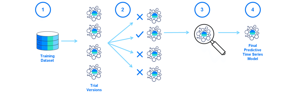
Smart Predict uses the training and validation data sets and performs the following steps when creating a time series model for data partitioning:
- From the training data set, several trial versions of the time series model are trained.
- The best trial version of the time series model is selected.
- The trial version is evaluated using the validation set.
- The final predictive time series model is created.
Considerations When Creating a Time Series Forecasting Model
There are a few considerations to take into account when creating your time series forecasting model:
1. Scale of the predictions:Consider the scale of the predictions. For example, if historical data is captured every month, week, day, hour, or minute, then the predictions will be produced in the same unit of time. Therefore, if data values are recorded every month, it is not meaningful to request predictions for the next few days. If data is recorded every minute by sensors, but the minute is not relevant for the use case, then a higher unit of time such as hour should be used.
2. Aggregation:Consider the aggregation of data in the unit of time required and define an aggregation function.
- For example, an aggregation function could calculate one value for the hour from the 60 values measured for each of the 60 minutes of this hour. It can be the first value, the last value, the mid-value, or a calculated value. For example, the average or a more complex formula.
- An important point to keep in mind is the size of the aggregation. A large aggregation may hide information and decrease the quality of the predictions. However, an appropriate aggregation smooths the signal when there is a lot of noise. Test and experiment to choose the best aggregation function.
3. Sort the data:The historical data set must be cleaned so that each unit of time corresponds to only one value of the target variable. Smart Predict automatically sorts the data.
Use Case & Data
In this scenario, the goal is to predict sales for thousands of product families sold across Favorita stores in Ecuador. The training data consists of several key elements: dates, store and product details, promotional status of the items, and historical sales figures. Additionally, supplementary data files are available, offering extra insights that may enhance model accuracy and performance during the forecasting process.
The training dataset includes time series data for several features: store_nbr, family, on-promotion, and the target variable sales.
- store_nbrrepresents the store where the products are sold.
- familyrefers to the category or type of product sold.
- salesprovides the total sales for a product family at a specific store on a given date. Sales values can be fractional, as products may be sold in partial quantities (e.g., 1.5 kg of cheese versus 1 unit of a product like a bag of chips).
- on-promotionindicates the number of items within a product family that were part of a promotion at a given store on a particular date.
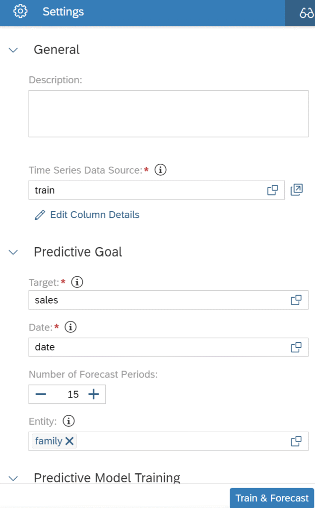
Entity: The nominal column(s) serve to identify each individual entity for which you aim to generate a forecast (e.g., forecasting sales for different countries). The predictive model analyzes the unique behavior associated with each entity and generates a separate forecast for each distinct combination of values within these columns.
Conclusion
In summary, time series forecasting within SAP SAC provides powerful insights that enable businesses to predict future trends based on historical data. By understanding key components such as trends, seasonality, and fluctuations, companies can make informed decisions that drive better outcomes.
Stay tuned for our upcoming discussion, where we’ll dive deeper into a practical use case, applying these concepts to forecast sales across product families at Favorita stores. We’ll explore how to leverage SAP SAC’s predictive capabilities to enhance forecasting accuracy and optimize business strategies.